Configuration moves from theory to device - HAL device that is. For those who have had just a bit of computer programming, this section is the ``Hello World'' of the HAL. As noted above halcmd can be used to create a working system. It is a command line or text file tool for configuration and tuning. The following examples illustrate its setup and operation.
Command line examples are presented in bold typewriter font. Responses from the computer will be in typewriter font. Text inside square brackets [like-this] is optional. Text inside angle brackets <like-this> represents a field that can take on different values, and the adjacent paragraph will explain the appropriate values. Text items separated by a vertical bar means that one or the other, but not both, should be present. All command line examples assume that you are in the emc2/ directory, and paths will be shown accordingly when needed.
RTAPI stands for Real Time Application Programming Interface. Many HAL components work in realtime, and all HAL components store data in shared memory so realtime components can access it. Normal Linux does not support realtime programming or the type of shared memory that HAL needs. Fortunately there are realtime operating systems (RTOS's) that provide the neccessary extensions to Linux. Unfortunately, each RTOS does things a little differently.
To address these differences, the EMC team came up with RTAPI, which provides a consistent way for programs to talk to the RTOS. If you are a programmer who wants to work on the internals of EMC, you may want to study emc2/src/rtapi/rtapi.h to understand the API. But if you are a normal person all you need to know about RTAPI is that it (and the RTOS) needs to be loaded into the memory of your computer before you do anything with HAL.
For this tutorial, we are going to assume that you have successfully compiled the emc2/ source tree. In that case, all you need to do is load the required RTOS and RTAPI modules into memory. Just run the following command:
Your version of halcmd may include tab-completion. Instead of completing filenames as a shell does, it completes commands with HAL identifiers. Try pressing tab after starting a HAL command:
For the first example, we will use a HAL component called siggen,
which is a simple signal generator. A complete description of the
siggen component can be found in section ![[*]](crossref.png) of this document. It is a realtime component, implemented as a Linux
kernel module. To load siggen use the halcmd loadrt
command:
of this document. It is a realtime component, implemented as a Linux
kernel module. To load siggen use the halcmd loadrt
command:
Now that the module is loaded, it is time to introduce halcmd,
the command line tool used to configure the HAL. This tutorial will
introduce some halcmd features, for a more complete description try
man halcmd, or see the halcmd reference in section
of this document. The first halcmd feature is the
show command. This command displays information about the current
state of the HAL. To show all installed components:
Next, let's see what pins siggen makes available:
The next step is to look at parameters:
Most realtime components export one or more functions to actually run the realtime code they contain. Let's see what function(s) siggen exported:
To actually run the code contained in the function siggen.0.update, we need a realtime thread. Eventually halcmd will have a newthread command that can be used to create a thread, but that requires some significant internal changes. For now, we have a component called threads that is used to create a new thread. Lets create a thread called test-thread with a period of 1mS (1000000nS):
The real power of HAL is that you can change things. For example, we can use the setp command to set the value of a parameter. Let's change the amplitude of the signal generator from 1.0 to 5.0:
emc2$
Most of what we have done with halcmd so far has simply been viewing things with the show command. However two of the commands actually changed things. As we design more complex systems with HAL, we will use many commands to configure things just the way we want them. HAL has the memory of an elephant, and will retain that configuration until we shut it down. But what about next time? We don't want to manually enter a bunch of commands every time we want to use the system. We can save the configuration of the entire HAL with a single command:
To restore the HAL configuration stored in saved.hal, we need to execute all of those HAL commands. To do that, we use halcmd -f <filename> which reads commands from a file:
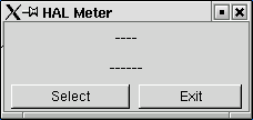
You can build very complex HAL systems without ever using a graphical interface. However there is something satisfying about seeing the result of your work. The first and simplest GUI tool for the HAL is halmeter. It is a very simple program that is the HAL equivalent of the handy Fluke multimeter (or Simpson analog meter for the old timers).
We will use the siggen component again to check out halmeter. If you just finished the previous example, then siggen is already loaded. If not, we can load it just like we did before:
At this point we have the siggen component loaded and running. It's time to start halmeter. Since halmeter is a GUI app, X must be running.
.
The meter in figure isn't very useful,
because it isn't displaying anything. To change that, click on the
'Select' button, which will open the probe selection dialog (figure
).
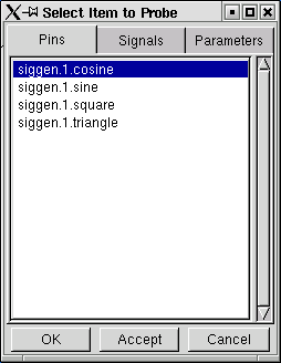
This dialog has three tabs. The first tab displays all of the HAL
pins in the system. The second one displays all the signals, and the
third displays all the parameters. We would like to look at the pin
siggen.0.triangle first, so click on it then click the 'OK'
button. The probe selection dialog will close, and the meter looks
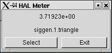
something like figure .
You should see the value changing as siggen generates its triangle wave. Halmeter refreshes its display about 5 times per second.
If you want to quickly look at a number of pins, you can use the 'Accept' button in the source selection dialog. Click on 'Select' to open the dialog again. This time, click on another pin, like siggen.0.cosine, and then click 'Accept'. When you click 'Accept', the meter immediately begins to display the newly selected item, but the dialog does not close. Try displaying a parameter instead of a pin. Click on the 'Parameters' tab, then select a parameter and click 'Accept' again. You can very quickly move the ``meter probes'' from one item to the next with a couple of clicks.
To shut down halmeter, just click the exit button.
If you want to look at more than one pin, signal, or parameter at a time, you can just start more halmeters. The halmeter window was intentionally made very small so you could have a lot of them on the screen at once. 1.3
Up till now we have only loaded one HAL component. But the whole idea behind the HAL is to allow you to load and connect a number of simple components to make up a complex system. The next example will use two components.
Before we can begin building this new example, we want to start with a clean slate. If you just finished one of the previous examples, we need to remove the all components and reload the RTAPI and HAL libraries:
Now we are going to load the step pulse generator component. For a
detailed description of this component refer to section .
For now, we can skip the details, and just run the following commands:1.4
As before, we can use halcmd show to take a look at the HAL. This time we have a lot more pins and parameters than before:
What we have is two step pulse generators, and a signal generator. Now it is time to create some HAL signals to connect the two components. We are going to pretend that the two step pulse generators are driving the X and Y axis of a machine. We want to move the table in circles. To do this, we will send a cosine signal to the X axis, and a sine signal to the Y axis. The siggen module creates the sine and cosine, but we need ``wires'' to connect the modules together. In the HAL, ``wires'' are called signals. We need to create two of them. We can call them anything we want, for this example they will be X_vel and Y_vel. To create them we use the the newsig command. We also need to specify the type of data that will flow through these ``wires'', in this case it is floating point:
halcmd: linksp Y_vel freqgen.1.velocity
Thinking about data flowing through ``wires'' makes pins and signals fairly easy to understand. Threads and functions are a little more difficult. Functions contain the computer instructions that actually get things done. Thread are the method used to make those instructions run when they are needed. First let's look at the functions available to us:
The other three functions are related to the step pulse generators:
The first one, freqgen.capture_position, is used for position feedback. It captures the value of an internal counter that counts the step pulses as they are generated. Assuming no missed steps, this counter indicates the position of the motor.
The main function for the step pulse generator is freqgen.make_pulses. Every time make_pulses runs it decides if it is time to take a step, and if so sets the outputs accordingly. For smooth step pulses, it should run as frequently as possible. Because it needs to run so fast, make_pulses is highly optimized and performs only a few calculations. Unlike the others, it does not need floating point math.
The last function, freqgen.update_freq, is responsible for doing scaling and some other calculations that need to be performed only when the frequency command changes.
What this means for our example is that we want to run siggen.0.update at a moderate rate to calculate the sine and cosine values. Immediately after we run siggen.0.update, we want to run freqgen.update_freq to load the new values into the step pulse generator. Finally we need to run freqgen.make_pulses as fast as possible for smooth pulses. Because we don't use position feedback, we don't need to run freqgen.capture_position at all.
We run functions by adding them to threads. Each thread runs at a specific rate. Let's see what threads we have available:
We are almost ready to start our HAL system. However we still need to adjust a few parameters. By default, the siggen component generates signals that swing from +1 to -1. For our example that is fine, we want the table speed to vary from +1 to -1 inches per second. However the scaling of the step pulse generator isn't quite right. By default, it generates an output frequency of 1 step per second with an input of 1.000. It is unlikely that one step per second will give us one inch per second of table movement. Let's assume instead that we have a 5 turn per inch leadscrew, connected to a 200 step per rev stepper with 10x microstepping. So it takes 2000 steps for one revolution of the screw, and 5 revolutions to travel one inch. that means the overall scaling is 10000 steps per inch. We need to multiply the velocity input to the step pulse generator by 10000 to get the proper output. That is exactly what the parameter freqgen.n.velocity-scale is for. In this case, both the X and Y axis have the same scaling, so we set the scaling parameters for both to 10000:
We now have everything configured and are ready to start it up. Just like in the first example, we use the start command:
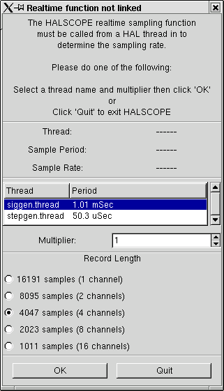
The previous example generates some very interesting signals. But much of what happens is far too fast to see with halmeter. To take a closer look at what is going on inside the HAL, we want an oscilloscope. Fortunately HAL has one, called halscope.
Halscope has two parts - a realtime part that is loaded as a kernel module, and a user part that supplies the GUI and display. However, you don't need to worry about this, because the userspace portion will automatically request that the realtime part be loaded.
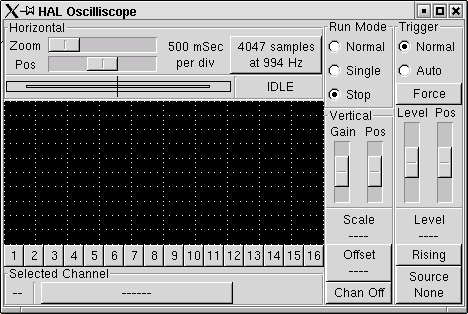
1.5.
This dialog is where you set the sampling rate for the oscilloscope.
For now we want to sample once per millisecond, so click on the 1.03mS
thread ``slow'' (formerly ``siggen.thread'', see footnote),
and leave the multiplier at 1. We will also leave the record length
at 4047 samples, so that we can use up to four channels at one time.
When you select a thread and then click ``OK'', the dialog disappears,
and the scope window looks something like figure .
At this point, Halscope is ready to use. We have already selected a sample rate and record length, so the next step is to decide what to look at. This is equivalent to hooking ``virtual scope probes'' to the HAL. Halscope has 16 channels, but the number you can use at any one time depends on the record length - more channels means shorter records, since the memory available for the record is fixed at approximately 16,000 samples.
The channel buttons run across the bottom of the halscope screen.
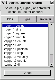
Click button ``1'', and you will see the ``Select Channel Source''
dialog, figure . This dialog is very similar
to the one used by Halmeter. We would like to look at the signals
we defined earlier, so we click on the ``Signals'' tab, and the
dialog displays all of the signals in the HAL (only two for this example).
To choose a signal, just click on it. In this case, we want to use channel 1 to display the signal ``X_vel''. When we click on ``X_vel'', the dialog closes and the channel is now selected. The channel 1 button is pressed in, and channel number 1 and the name ``X_vel'' appear below the row of buttons. That display always indicates the selected channel - you can have many channels on the screen, but the selected one is highlighted, and the various controls like vertical position and scale always work on the selected one. To add a signal to channel 2, click the ``2'' button. When the dialog pops up, click the ``Signals'' tab, then click on ``Y_vel''.
We also want to look at the square and triangle wave outputs. There are no signals connected to those pins, so we use the ``Pins'' tab instead. For channel 3, select ``siggen.0.triangle'' and for channel 4, select ``siggen.0.square''.
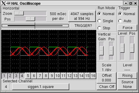
Now that we have several probes hooked to the HAL, it's time to capture
some waveforms. To start the scope, click the ``Normal'' button
in the ``Run Mode'' section of the screen (upper right). Since
we have a 4000 sample record length, and are acquiring 1000 samples
per second, it will take halscope about 2 seconds to fill half of
its buffer. During that time a progress bar just above the main screen
will show the buffer filling. Once the buffer is half full, the scope
waits for a trigger. Since we haven't configured one yet, it will
wait forever. To manually trigger it, click the ``Force'' button
in the ``Trigger'' section at the top right. You should see the
remainder of the buffer fill, then the screen will display the captured
waveforms. The result will look something like figure .
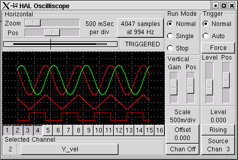
The ``Selected Channel'' box at the bottom tells you that the green trace is the currently selected one, channel 4, which is displaying the value of the pin ``siggen.1.square''. Try clicking channel buttons 1 through 3 to highlight the other three traces.
The traces are rather hard to distinguish since all four are on top
of each other. To fix this, we use the ``Vertical'' controls in
the box to the right of the screen. These controls act on the currently
selected channel. When adjusting the gain, notice that it covers a
huge range - unlike a real scope, this one can display signals ranging
from very tiny (pico-units) to very large (Tera-units). The position
control moves the displayed trace up and down over the height of the
screen only. For larger adjustments the offset button should be used
(see the halscope reference in section for details).
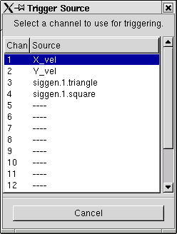
Using the ``Force'' button is a rather unsatisfying way to trigger
the scope. To set up real triggering, click on the ``Source''
button at the bottom right. It will pop up the ``Trigger Source''
dialog, which is simply a list of all the probes that are currently
connected (Figure ). Select a probe to
use for triggering by clicking on it. For this example we will use
channel 3, the triangle wave.
After setting the trigger source, you can adjust the trigger level and trigger position using the sliders in the ``Trigger'' box along the right edge. The level can be adjusted from the top to the bottom of the screen, and is displayed below the sliders. The position is the location of the trigger point within the overall record. With the slider all the way down, the trigger point is at the end of the record, and halscope displays what happened before the trigger point. When the slider is all the way up, the trigger point is at the beginning of the record, displaying what happened after it was triggered. The trigger point is visible as a vertical line in the progress box above the screen. The trigger polarity can be changed by clicking the button just below the trigger level display. Note that changing the trigger position stops the scope, once the position is adjusted you restart the scope by clicking the ``Normal'' button in the ``Run Mode'' box.
Now that we have adjusted the vertical controls and triggering, the
scope display looks something like figure .
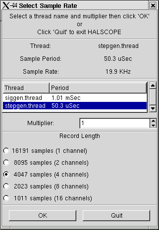
To look closely at part of a waveform, you can use the zoom slider at the top of the screen to expand the waveforms horizontally, and the position slider to determine which part of the zoomed waveform is visible. However, sometimes simply expanding the waveforms isn't enough and you need to increase the sampling rate. For example, we would like to look at the actual step pulses that are being generated in our example. Since the step pulses may be only 50uS long, sampling at 1KHz isn't fast enough. To change the sample rate, click on the button that displays the record length and sample rate to bring up the ``Select Sample Rate'' dialog, figure . For this example, we will click on the 50uS thread, ``fast'', which gives us a sample rate of about 20KHz. Now instead of displaying about 4 seconds worth of data, one record is 4000 samples at 20KHz, or about 0.20 seconds.
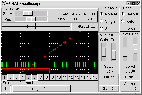
Now let's look at the step pulses. Halscope has 16 channels, but for
this example we are using only 4 at a time. Before we select any more
channels, we need to turn off a couple. Click on the channel 2 button,
then click the ``Off'' button at the bottom of the ``Vertical''
box. Then click on channel 3, turn if off, and do the same for channel
4. Even though the channels are turned off, they still remember what
they are connected to, and in fact we will continue to use channel
3 as the trigger source. To add new channels, select channel 5, and
choose pin ``stepgen.1.dir'', then channel 6, and select ``stepgen.1.step''.
Then click run mode ``Normal'' to start the scope, and adjust
the horizontal zoom to 5mS per division. You should see the step pulses
slow down as the velocity command (channel 1) approaches zero, then
the direction pin changes state and the step pulses speed up again.
You might want to increase the gain on channel 1 to about 20m per
division to better see the change in the velocity command. The result
should look like figure .